03 · Enformer: Sequence-to-Epigenome with CNNs + Transformers
GENE 46100 — Unit 02
2026-05-05
Enformer: the model
Input: 196,608 bp of DNA sequence (one-hot encoded)
Output: Predicted signal at 896 genomic bins for:
- 5,313 human epigenomic tracks (CAGE, DNase-seq, ChIP-seq)
- 1,643 mouse epigenomic tracks
Architecture: CNN stem → convolutional tower → transformer → prediction heads
Key innovation: Transformer attention captures enhancer–promoter interactions across the full 200 kb window.
Overview: five stages
Input (B, 196608, 4)
       ↓
  [1] Stem                Conv1d + residual + softmax pool   → (B, 768, 98304)
       ↓
  [2] Conv Tower          6 stages, expanding channels       → (B, 1536, 1536)
       ↓
  [3] Transformer         11 layers, relative attention      → (B, 1536, 1536)
       ↓
  [4] Crop + Pointwise    center crop + expand dim           → (B, 896, 3072)
       ↓
  [5] Prediction Heads    per-species linear + Softplus      → (B, 896, 5313)
Total sequence compression: 128× (196,608 → 1,536 positions before crop)
Architecture diagram
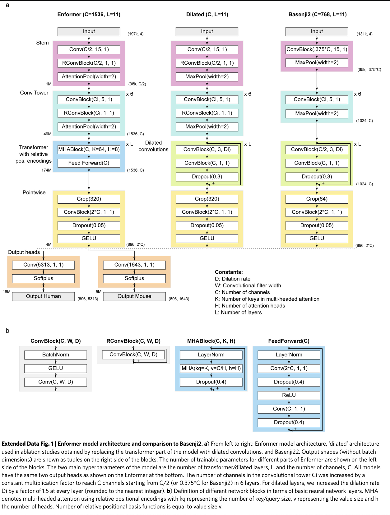
Block definitions
Three building blocks appear throughout:
ConvBlock(C, k)
BatchNorm1d
    ↓
  GELU
    ↓
Conv1d(C, kernel=k, padding=same)
RConvBlock(C, k)
x + ConvBlock(C, k) ← residualSoftmaxPool(n)
For each window of n adjacent positions, learn a per-channel attention weight and take the weighted sum.
Better than max pooling (keeps information from both positions) and average pooling (can focus).
Halves sequence length.
Stage 1: Stem
Input (B, 196608, 4)
    ↓  Rearrange → (B, 4, 196608)
    ↓  Conv1d(4→768, kernel=15)
    ↓  RConvBlock(768, kernel=1)
    ↓  SoftmaxPool(2)
Output (B, 768, 98304)
Design choices:
- kernel=15: wide enough to detect TF binding motifs (6–20 bp)
- RConvBlock(k=1): pointwise channel mixing without expanding receptive field
- SoftmaxPool: first 2× downsampling
- Works at half the final channel width (768, not 1536)
Stage 2: Convolutional Tower
Six identical-structure stages:
ConvBlock(Cᵢ→Cᵢ₊₁, kernel=5)   ← no residual
    ↓
RConvBlock(Cᵢ₊₁, kernel=1)      ← with residual
    ↓
SoftmaxPool(2)                   ← halve length
Channel progression (geometric, rounded to 128):
768 → 896 → 1024 → 1152 → 1280 → 1536
After stem + 6 stages:
| Stage | Channels | Sequence |
|---|---|---|
| Stem out | 768 | 98,304 |
| Stage 1 | 768 | 49,152 |
| Stage 2 | 896 | 24,576 |
| Stage 3 | 1024 | 12,288 |
| Stage 4 | 1152 | 6,144 |
| Stage 5 | 1280 | 3,072 |
| Stage 6 | 1536 | 1,536 |
Conv Tower: what it learns
Local → abstract hierarchy:
- Early layers: individual nucleotides, simple motifs
- Mid layers: composite motifs, chromatin states
- Late layers: regulatory module signatures
Each pooling step doubles the genomic span each unit sees.
By stage 6, each of the 1,536 positions represents 128 bp of original sequence.
Why geometric channel growth?
channels ∝ base^stage
Constant ratio between stages — a principled inductive bias that larger feature spaces are needed as representations become more abstract.
Why no residual on the k=5 conv?
Channel dimensions change between stages (in ≠ out), so a skip connection isn’t possible there.
Stage 3: Transformer
11 layers. Input rearranged to (B, 1536 positions, 1536 dim).
Each layer:
LayerNorm
  → MultiHeadAttention (8 heads)
  → Dropout(0.4)
[+ residual]

LayerNorm
  → Linear(1536→3072) → Dropout(0.4) → ReLU
  → Linear(3072→1536) → Dropout(0.4)
[+ residual]
Attention dimensions:
| Heads | 8 |
| Key dim | 64 per head |
| Value dim | 192 per head |
Key/query dim (64) < value dim (192): keys determine where to attend; values carry what to mix.
Output projection is zero-initialized → each layer starts as identity.
Relative positional encoding
Why not absolute position?
An enhancer 50 kb upstream has the same effect regardless of where in the genome it sits. What matters is relative distance between positions.
The attention logit for position \(i\) attending to \(j\):
\[\text{logit}(i,j) = \underbrace{(q_i + b_c) \cdot k_j}_{\text{content}} + \underbrace{(q_i + b_p) \cdot r_{j-i}}_{\text{position}}\]
\(r_{j-i}\) is a learned encoding of the distance \(j-i\).
Relative positional encoding: distance basis functions
Three basis functions encode \(r_{j-i}\):
Exponential decay
Nearby positions matter more. 64 scales from fine to coarse.
Central mask
Step functions: “within k positions?” Binary windows of increasing width.
Gamma PDF
Peaked functions. Can encode “matters most at distance X.”
Together: rich vocabulary of distance relationships, learned from data.
At 1,536 positions × 128 bp/position: attention between positions 0 and 1,535 spans the full 196,608 bp window — capturing enhancer–promoter interactions impossible for the CNN alone.
Stage 4: Crop + Pointwise
Center crop: 1,536 → 896 positions
Remove 320 positions from each endEdge positions have asymmetric context — they can’t “see” past the sequence boundary. The central 896 positions have full, symmetric context on both sides.
In genomic coordinates: 896 × 128 bp = 114,688 bp of predictions from a 196,608 bp input.
Pointwise projection: 1,536 → 3,072
Linear(1536→3072)
  → Dropout(0.05)
  → GELU
Expands the shared representation before species-specific heads. Lower dropout (0.05 vs 0.4) — we’re close to the output.
Stage 5: Prediction Heads
Human head:
  Linear(3072→5,313) → Softplus

Mouse head:
  Linear(3072→1,643) → Softplus
Applied independently at each of the 896 positions.
The trunk is fully shared between species. Only the final linear layers differ.
Why Softplus?
Epigenomic signals are non-negative counts.
- ReLU: non-negative ✓, but zero gradient for negative inputs ✗
- Softplus = log(1 + eˣ): non-negative ✓, smooth ✓, gradient everywhere ✓
Why train on two species?
Joint training forces the trunk to learn conserved regulatory grammar. Features that matter in both human and mouse are more likely to be biologically real.
Full shape summary
| Stage | Output shape |
|---|---|
| Input | (B, 196608, 4) |
| Stem | (B, 768, 98304) |
| Conv Tower | (B, 1536, 1536) |
| Transformer | (B, 1536, 1536) |
| Center crop | (B, 896, 1536) |
| Pointwise | (B, 896, 3072) |
| Human head | (B, 896, 5313) |
Part 3: Loss Function
Why Poisson NLL?
What are we predicting?
Epigenomic tracks are read counts from sequencing:
- ChIP-seq: reads mapping to each 128 bp bin
- CAGE: reads at each TSS bin
- DNase-seq: reads in accessible regions
Count data is naturally modeled as Poisson distributed.
Poisson distribution:
\[P(y \mid \lambda) = \frac{e^{-\lambda} \lambda^y}{y!}\]
- \(\lambda\): predicted rate (Softplus output)
- \(y\): observed count
Poisson NLL loss:
\[\mathcal{L} = \lambda - y \log \lambda + \text{const}\]
Penalizes overestimating sparse tracks heavily. Scales naturally with signal magnitude.
Rule of thumb: when targets are non-negative counts with variance ≈ mean, use Poisson NLL. MSE would underweight high-count bins and treat all errors equally regardless of scale.
Part 4: Data & Augmentation
Training data
Human: 5,313 tracks
- CAGE (transcription start site activity)
- DNase-seq (open chromatin / accessibility)
- ChIP-seq — histone marks: H3K27ac, H3K4me1, H3K4me3, H3K36me3, …
- ChIP-seq — TF binding: CTCF, POLR2A, …
Sources: ENCODE, Roadmap Epigenomics, GEO
Mouse: 1,643 tracks
Same assay types, profiled in mouse tissues.
Data format:
- HDF5 files
- One-hot encoded sequences: shape (L, 4)
- Target values: shape (896, N_tracks)
- Pre-split into train / validation / test chromosomes
Augmentation 1: Sequence shift
What: randomly shift the input sequence by ±1–4 bp, re-center the prediction window.
Original:  [----196,608 bp----]
                 ↓ predict
           [------896 bins-----]

Shifted+3: [---196,608 bp---]
                 ↓ predict
             [----896 bins----]
Why:
- The model shouldn’t care whether a motif falls at position 1,000 or 1,003
- Shift augmentation teaches translation invariance at the nucleotide level
- Especially important because the conv tower compresses by 128×: a 1 bp shift is sub-resolution without augmentation
Augmentation 2: Reverse complement
What: flip the sequence strand.
Forward:  5'–ACGT...ACGT–3'
Reverse complement:
          3'–TGCA...TGCA–5'
             ↕ reverse ↕
          5'–ACGT...TGCA–3'
Applied by: 1. Reversing the sequence order 2. Swapping A↔︎T and C↔︎G (complement)
Why:
- DNA is double-stranded — the same gene exists on both strands
- TF binding motifs are often palindromic, but not always
- The model must learn to recognize regulatory elements regardless of strand orientation
- Also doubles the effective training set size
Both augmentations exploit known biological symmetries. The model doesn’t need to learn “this motif on the + strand is different from the same motif on the − strand” — that’s baked in.
Summary
Architecture:
- Stem: motif detection, 2× compression
- Conv Tower: hierarchical features, 64× compression (6 stages)
- Transformer: long-range regulatory interactions (up to 196 kb)
- Heads: per-species predictions, Softplus output
Training:
- Loss: Poisson NLL — right for count data
- Augmentation: shift (±4 bp) + reverse complement
- Multi-species: joint human + mouse training for regularization
- Targets: 5,313 human + 1,643 mouse epigenomic tracks
GENE 46100 · Deep Learning in Genomics