03 · DNA Sequence Scoring with CNNs

Jupyter notebook in Colab

Note: If the notebook doesn’t render correctly, click Open with → Google Colaboratory in the top-right of the Google Drive preview.

Originally created by Erin Wilson (source). Adapted by Haky Im and Ran Blekhman for GENE 46100.

Building on notebook-02

In notebook-02 you built a CNN that detects a spike pattern in a numeric signal. This notebook applies the same architecture to DNA sequences. The key differences:

	Notebook-02	This notebook
Input	1-channel numeric signal	4-channel one-hot DNA (A/C/G/T)
Task	Classification (spike yes/no)	Regression (predict a score)
Pattern	Fixed spike shape	Sequence motifs (TAT, GCG)
Batching	Full dataset in one pass	Mini-batches via DataLoader
Filters reveal	Spike-shaped weight vectors	Sequence logos

Everything else — Conv1d, ReLU, pooling, the training loop, filter visualization — carries over directly.

Install and load packages

if False:
    %pip install seaborn matplotlib logomaker
    %pip install scikit-learn plotnine tqdm pandas numpy
    %pip install torch torchvision torchmetrics

from collections import defaultdict
from itertools import product
import matplotlib.pyplot as plt
import numpy as np
import pandas as pd
import random
import torch
from torch import nn
import torch.nn.functional as F
from sklearn.model_selection import train_test_split

if torch.backends.mps.is_available():
    torch.set_default_dtype(torch.float32)
    print("Set default to float32 for MPS compatibility")

Set default to float32 for MPS compatibility

def set_seed(seed: int = 42) -> None:
    """Set random seeds for reproducibility across all libraries."""
    np.random.seed(seed)
    random.seed(seed)
    torch.manual_seed(seed)
    if torch.backends.mps.is_available():
        torch.mps.manual_seed(seed)
    elif torch.cuda.is_available():
        torch.cuda.manual_seed(seed)
        torch.backends.cudnn.deterministic = True
        torch.backends.cudnn.benchmark = False
    print(f"Random seed set as {seed}")

set_seed(17)

Random seed set as 17

Choose the best available device — GPU training is faster but the dataset here is small enough for CPU.

DEVICE = torch.device('mps' if torch.backends.mps.is_available()
                     else 'cuda' if torch.cuda.is_available()
                     else 'cpu')
DEVICE

device(type='mps')

Part 1: Generate Synthetic DNA Data

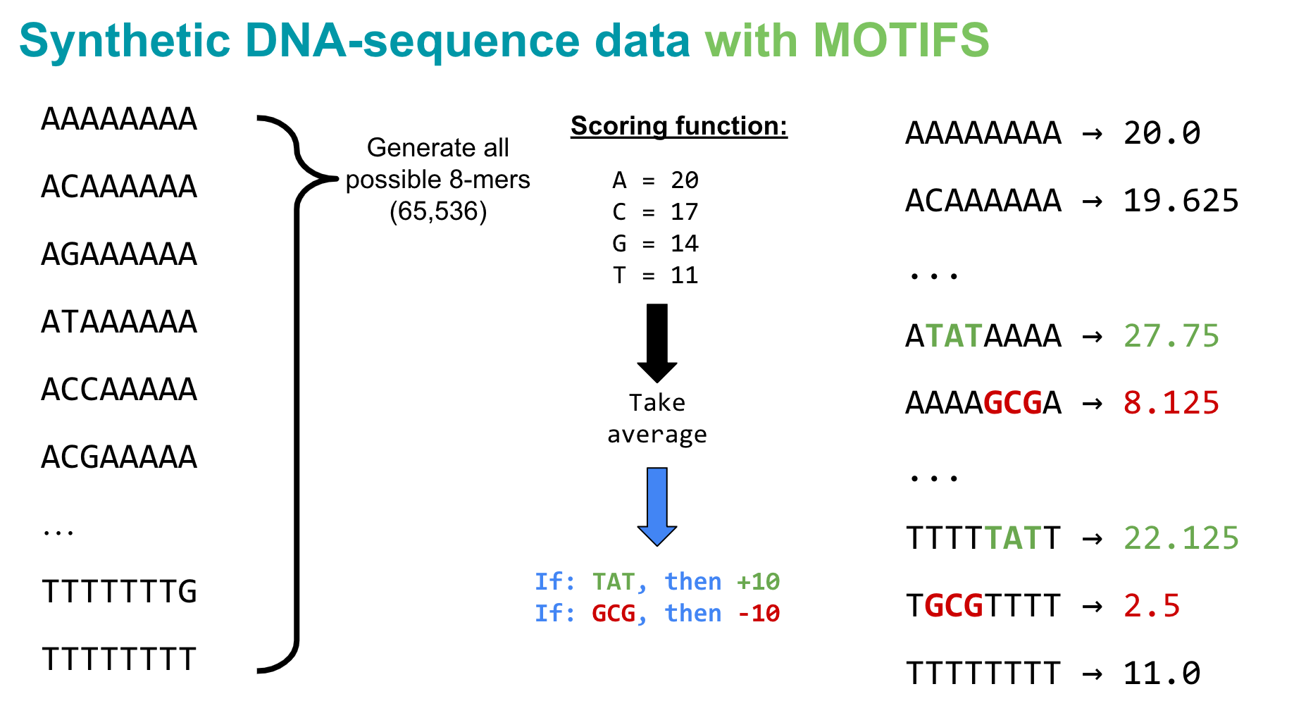
In real applications, we’d predict binding scores, expression levels, or chromatin accessibility from DNA. Here we design a simple scoring rule so we can verify that our PyTorch pipeline works before scaling to real biology.

Scoring rule for 8-mers:

• Each nucleotide contributes a base score: A = 20, C = 17, G = 14, T = 11
• The sequence score is the mean of its nucleotide scores
• Motif bonus: +10 if TAT appears anywhere, −10 if GCG appears

This creates three groups of sequences (no motif, TAT, GCG) — easy for us to inspect, and it tests whether the model can learn local patterns (motifs) beyond single-nucleotide effects.

def kmers(k):
    """Generate all possible k-mers of length k."""
    return [''.join(x) for x in product(['A','C','G','T'], repeat=k)]

seqs8 = kmers(8)
print('Total 8-mers:', len(seqs8))

Total 8-mers: 65536

score_dict = {'A': 20, 'C': 17, 'G': 14, 'T': 11}

def score_seqs_motif(seqs):
    """Score each sequence: mean nucleotide score ± motif bonuses."""
    data = []
    for seq in seqs:
        score = np.mean([score_dict[base] for base in seq], dtype=np.float32)
        if 'TAT' in seq:
            score += 10
        if 'GCG' in seq:
            score -= 10
        data.append([seq, score])
    return pd.DataFrame(data, columns=['seq', 'score'])

mer8 = score_seqs_motif(seqs8)
mer8.head()

	seq	score
0	AAAAAAAA	20.000
1	AAAAAAAC	19.625
2	AAAAAAAG	19.250
3	AAAAAAAT	18.875
4	AAAAAACA	19.625

Spot-check a few sequences with motifs to confirm the scoring logic:

mer8[mer8['seq'].isin(['TGCGTTTT', 'CCCCCTAT'])]

	seq	score
21875	CCCCCTAT	25.875
59135	TGCGTTTT	2.500

Visualize the score distribution

Discuss: The three-peaked histogram confirms our scoring rule: center peak (no motif), right peak (TAT bonus), left peak (GCG penalty).

plt.hist(mer8['score'].values, bins=20)
plt.title("8-mer score distribution")
plt.xlabel("Sequence score", fontsize=14)
plt.ylabel("Count", fontsize=14)
plt.show()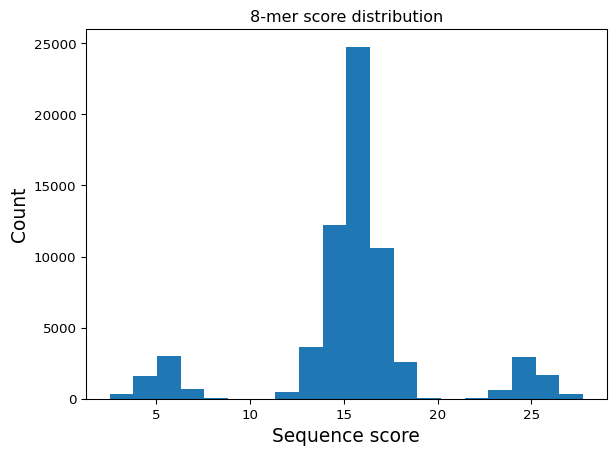

Question 1

Modify the scoring function to create a more complex pattern. Instead of giving fixed bonuses for “TAT” and “GCG”, implement a position-dependent scoring where a motif gets a higher bonus if it appears at the beginning of the sequence compared to the end. How does this change the distribution of scores?

Part 2: Prepare Data for PyTorch

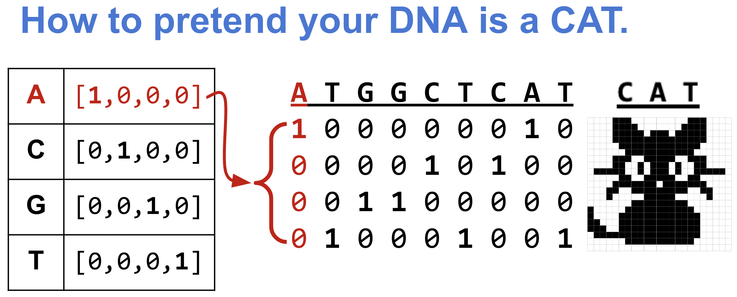
One-hot encoding: turning DNA into numbers

In notebook-02, our input was a 1-channel numeric signal. DNA is a string of letters, so we need to convert it. A naive approach — encoding A=0, C=1, G=2, T=3 — would imply a false ordering (A < C < G < T). No base is “more than” another. One-hot encoding avoids this by mapping each nucleotide to a unit vector in 4D space, making all bases equidistant:

• A → [1, 0, 0, 0], C → [0, 1, 0, 0], G → [0, 0, 1, 0], T → [0, 0, 0, 1]

An 8-mer becomes an (8 × 4) matrix — equivalent to a 4-channel signal of length 8. This is exactly the input shape Conv1d expects, with in_channels=4 instead of in_channels=1.

def one_hot_encode(seq):
    """One-hot encode a DNA sequence into a (seq_len, 4) numpy array."""
    allowed = set("ACTGN")
    if not set(seq).issubset(allowed):
        invalid = set(seq) - allowed
        raise ValueError(f"Invalid characters in sequence: {invalid}")

    nuc_d = {'A': [1.0, 0.0, 0.0, 0.0],
             'C': [0.0, 1.0, 0.0, 0.0],
             'G': [0.0, 0.0, 1.0, 0.0],
             'T': [0.0, 0.0, 0.0, 1.0],
             'N': [0.0, 0.0, 0.0, 0.0]}

    return np.array([nuc_d[x] for x in seq], dtype=np.float32)

print("AAAAAAAA:\n", one_hot_encode("AAAAAAAA"))

AAAAAAAA:
 [[1. 0. 0. 0.]
 [1. 0. 0. 0.]
 [1. 0. 0. 0.]
 [1. 0. 0. 0.]
 [1. 0. 0. 0.]
 [1. 0. 0. 0.]
 [1. 0. 0. 0.]
 [1. 0. 0. 0.]]

s = one_hot_encode("AGGTACCT")
print("AGGTACCT:\n", s)
print("Shape:", s.shape)

AGGTACCT:
 [[1. 0. 0. 0.]
 [0. 0. 1. 0.]
 [0. 0. 1. 0.]
 [0. 0. 0. 1.]
 [1. 0. 0. 0.]
 [0. 1. 0. 0.]
 [0. 1. 0. 0.]
 [0. 0. 0. 1.]]
Shape: (8, 4)

Train / validation / test split

We use the same train_test_split from sklearn as in notebook-02. The split ratios (64% train, 16% val, 20% test) ensure each set contains examples from all three score groups.

train_df, test_df = train_test_split(mer8, test_size=0.2, random_state=42)
train_df, val_df = train_test_split(train_df, test_size=0.2, random_state=42)

print("Train:", train_df.shape)
print("Val:  ", val_df.shape)
print("Test: ", test_df.shape)

Train: (41942, 2)
Val:   (10486, 2)
Test:  (13108, 2)

Verify that train, val, and test sets cover the full score distribution:

def plot_train_test_hist(train_df, val_df, test_df, bins=20):
    plt.hist(train_df['score'].values, bins=bins, label='train', alpha=0.5)
    plt.hist(val_df['score'].values, bins=bins, label='val', alpha=0.75)
    plt.hist(test_df['score'].values, bins=bins, label='test', alpha=0.4)
    plt.legend()
    plt.xlabel("Sequence score", fontsize=14)
    plt.ylabel("Count", fontsize=14)
    plt.show()

plot_train_test_hist(train_df, val_df, test_df)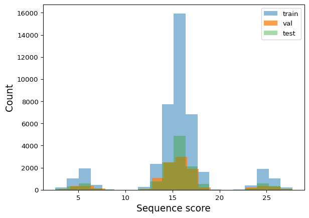

Dataset and DataLoader

In notebook-02 we passed the entire dataset as one tensor. With larger datasets that won’t fit in memory, so PyTorch provides Dataset (defines how to fetch one sample) and DataLoader (handles batching, shuffling, and parallel loading). This is the standard pattern you’ll see in every PyTorch project.

from torch.utils.data import Dataset, DataLoader

class SeqDatasetOHE(Dataset):
    """Dataset that one-hot encodes DNA sequences on construction."""
    def __init__(self, df, seq_col='seq', target_col='score'):
        self.seqs = list(df[seq_col].values)
        self.seq_len = len(self.seqs[0])
        self.ohe_seqs = torch.stack([torch.tensor(one_hot_encode(x)) for x in self.seqs])
        self.labels = torch.tensor(list(df[target_col].values)).unsqueeze(1)

    def __len__(self):
        return len(self.seqs)

    def __getitem__(self, idx):
        return self.ohe_seqs[idx], self.labels[idx]

def build_dataloaders(train_df, test_df, seq_col='seq', target_col='score',
                      batch_size=128, shuffle=True):
    """Create DataLoaders from train and test DataFrames."""
    train_ds = SeqDatasetOHE(train_df, seq_col=seq_col, target_col=target_col)
    test_ds = SeqDatasetOHE(test_df, seq_col=seq_col, target_col=target_col)
    train_dl = DataLoader(train_ds, batch_size=batch_size, shuffle=shuffle)
    test_dl = DataLoader(test_ds, batch_size=batch_size)
    return train_dl, test_dl

train_dl, val_dl = build_dataloaders(train_df, val_df)

Part 3: Define the Models

We compare two architectures to see why convolution matters for motif detection:

• Linear model — learns a weight for each nucleotide at each position. It can capture single-nucleotide effects (e.g. “A contributes +20”) but cannot detect motifs, because it has no way to recognize that specific adjacent nucleotides matter.
• CNN model — uses sliding filters of width 3, exactly the length of our motifs (TAT, GCG). Each filter can learn a local pattern regardless of where it appears — the same translation invariance from notebook-02. In fact, a CNN filter sliding over one-hot DNA is mathematically equivalent to scoring with a Position Weight Matrix (PWM) — but the weights are learned from data, not hand-designed.

class DNA_Linear(nn.Module):
    def __init__(self, seq_len):
        super().__init__()
        self.seq_len = seq_len
        self.lin = nn.Linear(4 * seq_len, 1)

    def forward(self, xb):
        xb = xb.view(xb.shape[0], self.seq_len * 4)
        return self.lin(xb)


class DNA_CNN(nn.Module):
    def __init__(self, seq_len, num_filters=32, kernel_size=3):
        super().__init__()
        self.seq_len = seq_len
        self.conv = nn.Conv1d(4, num_filters, kernel_size=kernel_size)
        self.relu = nn.ReLU(inplace=True)
        self.linear = nn.Linear(num_filters * (seq_len - kernel_size + 1), 1)

    def forward(self, xb):
        xb = xb.permute(0, 2, 1)   # (batch, seq_len, 4) → (batch, 4, seq_len)
        x = self.relu(self.conv(xb))
        x = x.flatten(1)
        return self.linear(x)

Part 4: Training Loop

The training loop follows the same structure as notebook-02 — forward pass, compute loss, backpropagate, update weights — but now processes mini-batches from the DataLoader instead of the full dataset at once.

We use MSE loss (regression) instead of cross-entropy (classification), and SGD as the optimizer.

def train_model(model, train_dl, val_dl, device, lr=0.01, epochs=50):
    """Train a model and return loss histories."""
    optimizer = torch.optim.SGD(model.parameters(), lr=lr)
    loss_fn = nn.MSELoss()
    train_losses, val_losses = [], []

    for epoch in range(epochs):
        # --- Training ---
        model.train()                      # enable training mode (affects dropout, batchnorm)
        batch_losses, batch_sizes = [], []
        for xb, yb in train_dl:
            xb, yb = xb.to(device), yb.to(device)  # move batch to GPU/CPU
            pred = model(xb.float())       # forward pass: input → prediction
            loss = loss_fn(pred, yb.float())  # compute loss: how wrong are we?
            optimizer.zero_grad()          # clear gradients from previous batch
            loss.backward()                # backprop: compute gradient of loss w.r.t. weights
            optimizer.step()               # update weights using gradients
            batch_losses.append(loss.item())
            batch_sizes.append(len(xb))
        train_loss = np.average(batch_losses, weights=batch_sizes)
        train_losses.append(train_loss)

        # --- Validation (no gradient updates) ---
        model.eval()                       # disable training-only layers
        with torch.no_grad():              # skip gradient tracking (saves memory)
            vl, ns = [], []
            for xb, yb in val_dl:
                xb, yb = xb.to(device), yb.to(device)
                loss = loss_fn(model(xb.float()), yb.float())
                vl.append(loss.item())
                ns.append(len(xb))
        val_loss = np.average(vl, weights=ns)
        val_losses.append(val_loss)

        print(f"E{epoch} | train loss: {train_loss:.3f} | val loss: {val_loss:.3f}")

    return train_losses, val_losses

Part 5: Train and Compare

Linear model

seq_len = len(train_df['seq'].values[0])

model_lin = DNA_Linear(seq_len).type(torch.float32).to(DEVICE)
lin_train_losses, lin_val_losses = train_model(model_lin, train_dl, val_dl, DEVICE)

E0 | train loss: 21.318 | val loss: 13.230
E1 | train loss: 13.034 | val loss: 13.083
E2 | train loss: 12.978 | val loss: 13.090
E3 | train loss: 12.976 | val loss: 13.087
E4 | train loss: 12.976 | val loss: 13.101
E5 | train loss: 12.976 | val loss: 13.089
E6 | train loss: 12.975 | val loss: 13.093
E7 | train loss: 12.975 | val loss: 13.096
E8 | train loss: 12.975 | val loss: 13.095
E9 | train loss: 12.975 | val loss: 13.099
E10 | train loss: 12.974 | val loss: 13.088
E11 | train loss: 12.976 | val loss: 13.087
E12 | train loss: 12.974 | val loss: 13.091
E13 | train loss: 12.975 | val loss: 13.092
E14 | train loss: 12.976 | val loss: 13.089
E15 | train loss: 12.974 | val loss: 13.087
E16 | train loss: 12.974 | val loss: 13.102
E17 | train loss: 12.975 | val loss: 13.091
E18 | train loss: 12.977 | val loss: 13.087
E19 | train loss: 12.974 | val loss: 13.094
E20 | train loss: 12.975 | val loss: 13.095
E21 | train loss: 12.974 | val loss: 13.090
E22 | train loss: 12.974 | val loss: 13.097
E23 | train loss: 12.973 | val loss: 13.095
E24 | train loss: 12.975 | val loss: 13.104
E25 | train loss: 12.975 | val loss: 13.092
E26 | train loss: 12.975 | val loss: 13.089
E27 | train loss: 12.975 | val loss: 13.090
E28 | train loss: 12.977 | val loss: 13.087
E29 | train loss: 12.975 | val loss: 13.093
E30 | train loss: 12.973 | val loss: 13.099
E31 | train loss: 12.972 | val loss: 13.090
E32 | train loss: 12.976 | val loss: 13.091
E33 | train loss: 12.974 | val loss: 13.088
E34 | train loss: 12.975 | val loss: 13.090
E35 | train loss: 12.974 | val loss: 13.091
E36 | train loss: 12.976 | val loss: 13.089
E37 | train loss: 12.976 | val loss: 13.091
E38 | train loss: 12.974 | val loss: 13.100
E39 | train loss: 12.976 | val loss: 13.090
E40 | train loss: 12.975 | val loss: 13.103
E41 | train loss: 12.973 | val loss: 13.103
E42 | train loss: 12.975 | val loss: 13.101
E43 | train loss: 12.974 | val loss: 13.099
E44 | train loss: 12.975 | val loss: 13.090
E45 | train loss: 12.971 | val loss: 13.090
E46 | train loss: 12.975 | val loss: 13.088
E47 | train loss: 12.975 | val loss: 13.090
E48 | train loss: 12.976 | val loss: 13.093
E49 | train loss: 12.975 | val loss: 13.093

def quick_loss_plot(data_label_list, loss_type="MSE Loss"):
    for i, (train_data, test_data, label) in enumerate(data_label_list):
        plt.plot(train_data, linestyle='--', color=f"C{i}", label=f"{label} Train")
        plt.plot(test_data, color=f"C{i}", label=f"{label} Val", linewidth=3.0)
    plt.legend(bbox_to_anchor=(1, 1), loc='upper left')
    plt.ylabel(loss_type)
    plt.xlabel("Epoch")
    plt.show()

lin_data_label = (lin_train_losses, lin_val_losses, "Linear")
quick_loss_plot([lin_data_label])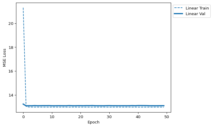

Discuss: The linear model plateaus quickly. This is an architecture problem, not an optimizer problem — no amount of tuning the learning rate will help. The model simply cannot represent motif-level patterns.

CNN model

model_cnn = DNA_CNN(seq_len).to(DEVICE)
cnn_train_losses, cnn_val_losses = train_model(model_cnn, train_dl, val_dl, DEVICE)

E0 | train loss: 14.492 | val loss: 10.484
E1 | train loss: 8.633 | val loss: 6.915
E2 | train loss: 6.223 | val loss: 5.235
E3 | train loss: 4.406 | val loss: 3.233
E4 | train loss: 2.966 | val loss: 2.395
E5 | train loss: 2.345 | val loss: 1.707
E6 | train loss: 1.971 | val loss: 1.153
E7 | train loss: 1.689 | val loss: 1.311
E8 | train loss: 1.640 | val loss: 1.509
E9 | train loss: 1.519 | val loss: 2.177
E10 | train loss: 1.343 | val loss: 0.944
E11 | train loss: 1.265 | val loss: 0.919
E12 | train loss: 1.234 | val loss: 0.890
E13 | train loss: 1.150 | val loss: 0.943
E14 | train loss: 1.117 | val loss: 0.912
E15 | train loss: 1.001 | val loss: 0.865
E16 | train loss: 1.077 | val loss: 1.094
E17 | train loss: 1.031 | val loss: 1.066
E18 | train loss: 1.024 | val loss: 0.901
E19 | train loss: 0.993 | val loss: 1.541
E20 | train loss: 1.043 | val loss: 1.124
E21 | train loss: 0.950 | val loss: 0.866
E22 | train loss: 0.948 | val loss: 0.877
E23 | train loss: 0.975 | val loss: 0.863
E24 | train loss: 0.984 | val loss: 0.957
E25 | train loss: 0.936 | val loss: 0.897
E26 | train loss: 0.938 | val loss: 0.879
E27 | train loss: 0.915 | val loss: 0.879
E28 | train loss: 0.964 | val loss: 1.019
E29 | train loss: 0.947 | val loss: 0.853
E30 | train loss: 0.937 | val loss: 0.875
E31 | train loss: 0.948 | val loss: 0.906
E32 | train loss: 0.938 | val loss: 0.998
E33 | train loss: 0.938 | val loss: 0.890
E34 | train loss: 0.908 | val loss: 0.910
E35 | train loss: 0.915 | val loss: 0.855
E36 | train loss: 0.896 | val loss: 0.859
E37 | train loss: 0.918 | val loss: 0.913
E38 | train loss: 0.896 | val loss: 0.849
E39 | train loss: 0.900 | val loss: 0.870
E40 | train loss: 0.898 | val loss: 0.871
E41 | train loss: 0.897 | val loss: 0.858
E42 | train loss: 0.912 | val loss: 0.890
E43 | train loss: 0.917 | val loss: 1.072
E44 | train loss: 0.938 | val loss: 0.880
E45 | train loss: 0.908 | val loss: 1.133
E46 | train loss: 0.902 | val loss: 1.000
E47 | train loss: 0.896 | val loss: 0.860
E48 | train loss: 0.908 | val loss: 0.863
E49 | train loss: 0.908 | val loss: 0.848

cnn_data_label = (cnn_train_losses, cnn_val_losses, "CNN")
quick_loss_plot([lin_data_label, cnn_data_label])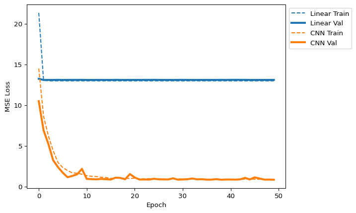

Discuss: The CNN loss drops much further — its sliding filters can capture the 3-mer motifs that the linear model cannot.

Spot-check predictions

Let’s compare what each model predicts for specific sequences to understand why the linear model fails:

oracle = dict(mer8[['seq', 'score']].values)

def quick_seq_pred(model, desc, seqs, oracle):
    print(f"__{desc}__")
    for dna in seqs:
        s = torch.tensor(one_hot_encode(dna)).unsqueeze(0).to(DEVICE)
        pred = model(s.float())
        actual = oracle[dna]
        diff = pred.item() - actual
        print(f"{dna}: pred:{pred.item():.3f} actual:{actual:.3f} ({diff:.3f})")

def quick_8mer_pred(model, oracle):
    groups = [
        ("poly-X seqs",      ['AAAAAAAA', 'CCCCCCCC', 'GGGGGGGG', 'TTTTTTTT']),
        ("other seqs",       ['AACCAACA', 'CCGGTGAG', 'GGGTAAGG', 'TTTCGTTT']),
        ("with TAT motif",   ['TATAAAAA', 'CCTATCCC', 'GTATGGGG', 'TTTATTTT']),
        ("with GCG motif",   ['AAGCGAAA', 'CGCGCCCC', 'GGGCGGGG', 'TTGCGTTT']),
        ("both TAT and GCG", ['ATATGCGA', 'TGCGTATT']),
    ]
    for desc, seqs in groups:
        quick_seq_pred(model, desc, seqs, oracle)
        print()

quick_8mer_pred(model_lin, oracle)

__poly-X seqs__
AAAAAAAA: pred:23.369 actual:20.000 (3.369)
CCCCCCCC: pred:13.739 actual:17.000 (-3.261)
GGGGGGGG: pred:7.075 actual:14.000 (-6.925)
TTTTTTTT: pred:17.852 actual:11.000 (6.852)

__other seqs__
AACCAACA: pred:18.908 actual:18.875 (0.033)
CCGGTGAG: pred:12.224 actual:15.125 (-2.901)
GGGTAAGG: pred:14.046 actual:15.125 (-1.079)
TTTCGTTT: pred:14.929 actual:12.125 (2.804)

__with TAT motif__
TATAAAAA: pred:22.251 actual:27.750 (-5.499)
CCTATCCC: pred:17.090 actual:25.875 (-8.785)
GTATGGGG: pred:12.320 actual:24.000 (-11.680)
TTTATTTT: pred:18.384 actual:22.125 (-3.741)

__with GCG motif__
AAGCGAAA: pred:16.918 actual:8.125 (8.793)
CGCGCCCC: pred:12.309 actual:6.250 (6.059)
GGGCGGGG: pred:8.108 actual:4.375 (3.733)
TTGCGTTT: pred:13.014 actual:2.500 (10.514)

__both TAT and GCG__
ATATGCGA: pred:15.878 actual:15.875 (0.003)
TGCGTATT: pred:14.738 actual:13.625 (1.113)

Discuss: The linear model underpredicts G-rich sequences and overpredicts T-rich ones. Why? It learned that G’s tend to appear in low-scoring sequences (because of GCG) and T’s in high-scoring ones (because of TAT). But it’s the 3-mer context that matters, not individual nucleotides — GCG is penalized while GAG is not. The linear model cannot make this distinction.

quick_8mer_pred(model_cnn, oracle)

__poly-X seqs__
AAAAAAAA: pred:19.958 actual:20.000 (-0.042)
CCCCCCCC: pred:16.993 actual:17.000 (-0.007)
GGGGGGGG: pred:13.848 actual:14.000 (-0.152)
TTTTTTTT: pred:11.030 actual:11.000 (0.030)

__other seqs__
AACCAACA: pred:18.884 actual:18.875 (0.009)
CCGGTGAG: pred:15.033 actual:15.125 (-0.092)
GGGTAAGG: pred:15.373 actual:15.125 (0.248)
TTTCGTTT: pred:12.051 actual:12.125 (-0.074)

__with TAT motif__
TATAAAAA: pred:26.473 actual:27.750 (-1.277)
CCTATCCC: pred:24.762 actual:25.875 (-1.113)
GTATGGGG: pred:23.085 actual:24.000 (-0.915)
TTTATTTT: pred:20.887 actual:22.125 (-1.238)

__with GCG motif__
AAGCGAAA: pred:9.226 actual:8.125 (1.101)
CGCGCCCC: pred:7.448 actual:6.250 (1.198)
GGGCGGGG: pred:5.434 actual:4.375 (1.059)
TTGCGTTT: pred:3.599 actual:2.500 (1.099)

__both TAT and GCG__
ATATGCGA: pred:15.430 actual:15.875 (-0.445)
TGCGTATT: pred:13.526 actual:13.625 (-0.099)

Discuss: The CNN handles both motif and non-motif sequences well, because its width-3 filters can detect the specific 3-mer patterns.

Question 2

Compare the performance of the Linear and CNN models by using different learning rates. First run both models with higher learning rates (0.05, 0.1) and lower learning rates (0.005, 0.001), then create loss plots showing:

• Linear model with these learning rates
• CNN model with these learning rates

Then analyze your results by answering:

1. How does changing the learning rate affect convergence for each model?
2. Which model is more sensitive to learning rate changes, and why?
3. Based on your analysis, what learning rate would you recommend for each model type, and why?

Part 6: Evaluate on Test Set

The test set was never seen during training — it’s our honest estimate of how the model would perform on new sequences.

import altair as alt
from sklearn.metrics import r2_score

def scatter_plot(model_name, df, r2):
    """Scatter actual vs predicted scores with a y=x reference line."""
    plt.scatter(df['truth'].values, df['pred'].values, alpha=0.2)
    xpoints = ypoints = plt.xlim()
    plt.plot(xpoints, ypoints, linestyle='--', color='k', lw=2, scalex=False, scaley=False)
    plt.ylim(xpoints)
    plt.ylabel("Predicted Score", fontsize=14)
    plt.xlabel("Actual Score", fontsize=14)
    plt.title(f"{model_name} (R² = {r2:.3f})", fontsize=20)
    plt.show()


def alt_scatter_plot(model_name, df, r2):
    """Interactive scatter plot with altair — hover to see sequences."""
    import os
    os.makedirs('alt_out', exist_ok=True)
    plot_df = pd.DataFrame({
        'truth': df['truth'].astype(float),
        'pred': df['pred'].astype(float),
        'seq': df['seq'].astype(str)
    })
    chart = alt.Chart(plot_df).mark_point().encode(
        x=alt.X('truth', type='quantitative', title='Actual Score'),
        y=alt.Y('pred', type='quantitative', title='Predicted Score'),
        tooltip=['seq']
    ).properties(title=f'{model_name} (R² = {r2:.3f})')
    chart.save(f'alt_out/scatter_plot_{model_name}.html')
    display(chart)


def scatter_pred(models, seqs, oracle, interactive=False):
    """Generate scatter plots for a list of (name, model) pairs."""
    for model_name, model in models:
        print(f"Running {model_name}")
        data = []
        for dna in seqs:
            s = torch.tensor(one_hot_encode(dna)).unsqueeze(0).to(DEVICE)
            actual = oracle[dna]
            pred = model(s.float())
            data.append([dna, actual, pred.item()])
        df = pd.DataFrame(data, columns=['seq', 'truth', 'pred'])
        r2 = r2_score(df['truth'], df['pred'])
        if interactive:
            alt_scatter_plot(model_name, df, r2)
        else:
            scatter_plot(model_name, df, r2)

seqs = test_df['seq'].values
models = [("Linear", model_lin), ("CNN", model_cnn)]
scatter_pred(models, seqs, oracle)

Running Linear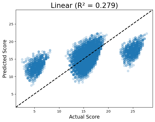

Running CNN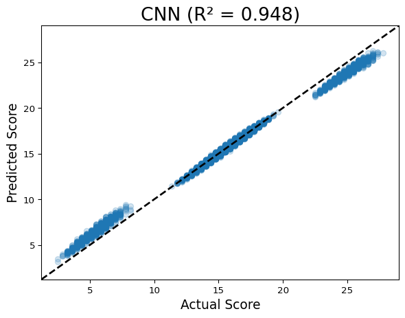

Discuss: In a perfect model, all points fall on the y=x line. The linear model shows three distinct bands (it can’t resolve within-band variation caused by motifs), while the CNN clusters tightly around the diagonal.

alt.data_transformers.disable_max_rows()
scatter_pred(models, seqs, oracle, interactive=True)

Running Linear

Running CNN

Discuss: Hover over outlier points in the interactive plot. The CNN’s largest errors tend to be sequences with multiple instances of a motif — our scoring function only gives one bonus regardless of count, but the model reasonably guesses that more motifs should mean a stronger effect.

Question 3

Design an approach to improve the model’s prediction accuracy, particularly focusing on the sequences where the current model performs poorly:

1. After identifying sequences where the CNN model has high prediction errors, propose and implement a modification to either the model architecture, the loss function, the training process, or the data representation
2. Retrain the model with your modifications
3. Create comparative visualizations (such as scatter plots, error histograms, or other appropriate plots) to demonstrate the impact of your changes
4. Analyze your results by discussing how your modification addresses the specific weaknesses you identified. What are the trade-offs involved in your approach?

Part 7: Visualize Convolutional Filters

In notebook-02 we plotted filter weights as bar charts. With DNA, we can go further: for each filter, we collect the subsequences that activate it most strongly, then display them as a sequence logo — the same representation used for transcription factor binding motifs.

Positions with tall letters have high information content (the filter is selective), while flat positions mean the filter doesn’t care which nucleotide appears there.

import logomaker

def get_conv_layers_from_model(model):
    """Extract convolutional layers and their weights from a model."""
    model_weights, conv_layers, bias_weights = [], [], []
    for child in model.children():
        if isinstance(child, nn.Conv1d):
            model_weights.append(child.weight)
            conv_layers.append(child)
            bias_weights.append(child.bias)
        elif isinstance(child, nn.Sequential):
            for subchild in child:
                if isinstance(subchild, nn.Conv1d):
                    model_weights.append(subchild.weight)
                    conv_layers.append(subchild)
                    bias_weights.append(subchild.bias)
    print(f"Total convolutional layers: {len(conv_layers)}")
    return conv_layers, model_weights, bias_weights


def view_filters(model_weights, num_cols=8):
    """Display raw filter weight heatmaps."""
    weights = model_weights[0]
    num_filt = weights.shape[0]
    filt_width = weights[0].shape[1]
    num_rows = int(np.ceil(num_filt / num_cols))

    plt.figure(figsize=(20, 17))
    for i, filt in enumerate(weights):
        ax = plt.subplot(num_rows, num_cols, i + 1)
        ax.imshow(filt.cpu().detach(), cmap='gray')
        ax.set_yticks(np.arange(4))
        ax.set_yticklabels(['A', 'C', 'G', 'T'])
        ax.set_xticks(np.arange(filt_width))
        ax.set_title(f"Filter {i}")
    plt.tight_layout()
    plt.show()

conv_layers, model_weights, bias_weights = get_conv_layers_from_model(model_cnn)
view_filters(model_weights)

Total convolutional layers: 1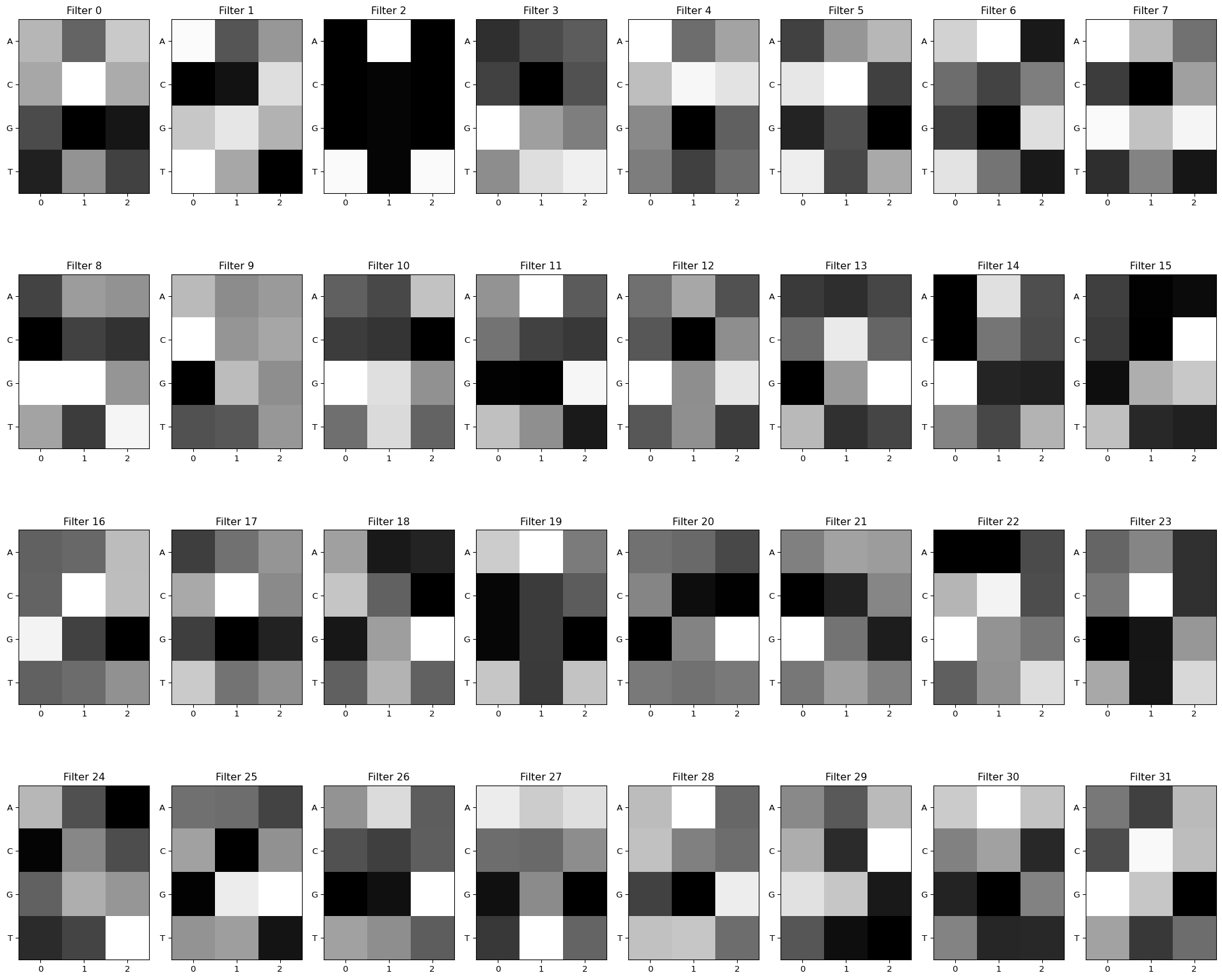

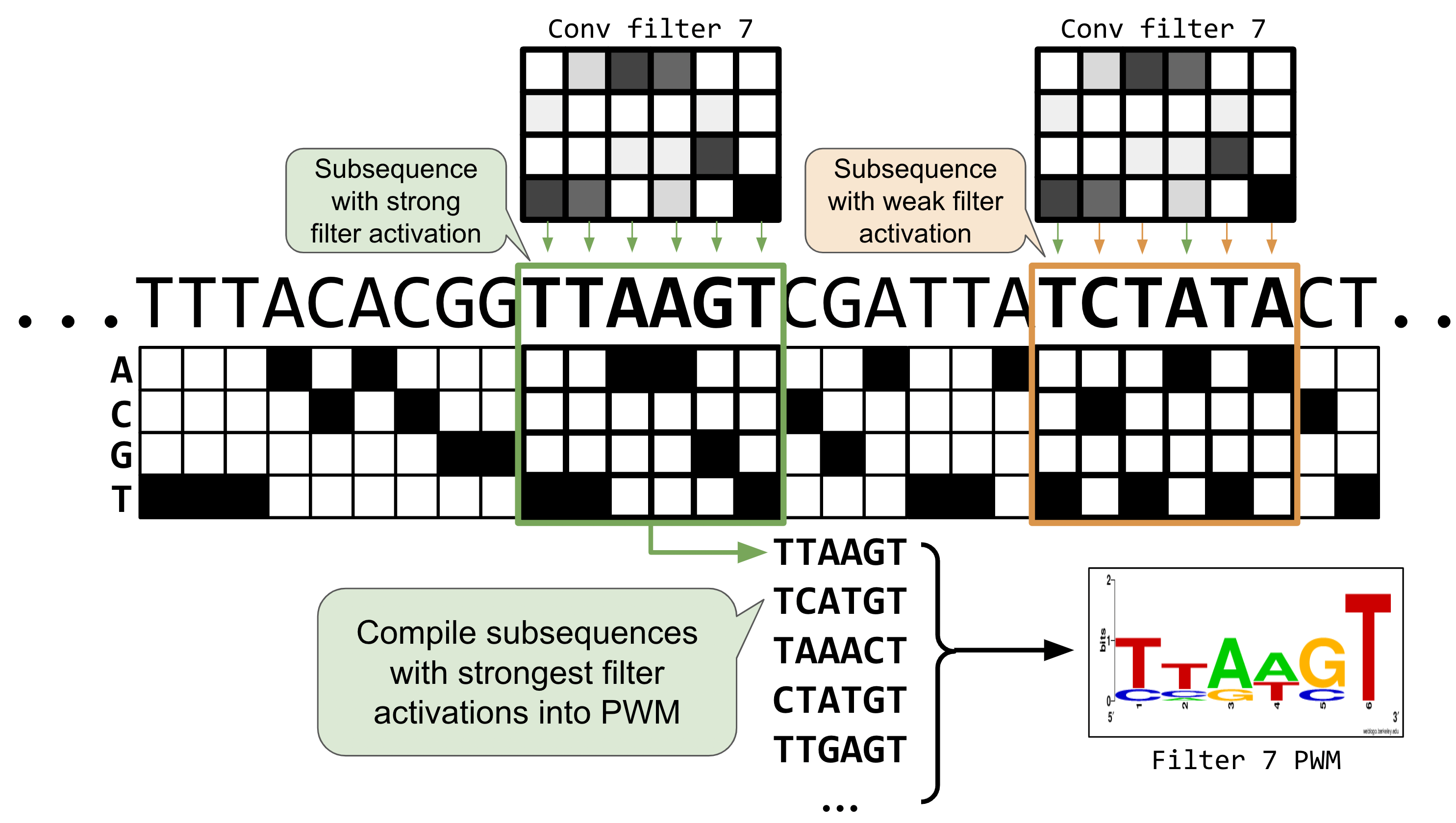
The raw heatmaps show what each filter “looks for,” but they’re hard to read. Let’s convert them to sequence logos by running test sequences through the filters and collecting which subsequences cause high activation:

def get_conv_output_for_seq(seq, conv_layer):
    """Run a sequence through a conv layer and return filter activations."""
    seq_t = torch.tensor(one_hot_encode(seq)).unsqueeze(0).permute(0, 2, 1).to(DEVICE)
    with torch.no_grad():
        return conv_layer(seq_t.float())[0]


def get_filter_activations(seqs, conv_layer, act_thresh=0):
    """Collect subsequences that activate each filter above a threshold,
    accumulating them into a count matrix (PWM) per filter."""
    num_filters = conv_layer.out_channels
    filt_width = conv_layer.kernel_size[0]
    filter_pwms = {i: torch.zeros(4, filt_width) for i in range(num_filters)}

    print(f"Num filters: {num_filters}, filter width: {filt_width}")

    for seq in seqs:
        res = get_conv_output_for_seq(seq, conv_layer)
        for filt_id, act_vec in enumerate(res):
            for pos in torch.where(act_vec > act_thresh)[0]:
                pos = pos.item()
                subseq = seq[pos:pos + filt_width]
                subseq_tensor = torch.tensor(one_hot_encode(subseq)).T
                filter_pwms[filt_id] += subseq_tensor

    return filter_pwms


def view_filters_and_logos(model_weights, filter_activations, num_cols=8):
    """Display filter heatmaps paired with their sequence logos."""
    weights = model_weights[0].squeeze(1)
    num_filts = len(filter_activations)
    num_rows = int(np.ceil(num_filts / num_cols)) * 2 + 1

    plt.figure(figsize=(20, 17))
    j = 0
    for i, filt in enumerate(weights):
        if i % num_cols == 0:
            j += num_cols

        ax1 = plt.subplot(num_rows, num_cols, i + j + 1)
        ax1.imshow(filt.cpu().detach(), cmap='gray')
        ax1.set_yticks(np.arange(4))
        ax1.set_yticklabels(['A', 'C', 'G', 'T'])
        ax1.set_xticks(np.arange(weights.shape[2]))
        ax1.set_title(f"Filter {i}")

        ax2 = plt.subplot(num_rows, num_cols, i + j + 1 + num_cols)
        filt_df = pd.DataFrame(filter_activations[i].T.numpy(), columns=['A', 'C', 'G', 'T'])
        filt_df_info = logomaker.transform_matrix(filt_df, from_type='counts', to_type='information')
        logo = logomaker.Logo(filt_df_info, ax=ax2)
        ax2.set_ylim(0, 2)
        ax2.set_title(f"Filter {i}")

    plt.tight_layout()

some_seqs = random.choices(seqs, k=3000)

filter_activations = get_filter_activations(some_seqs, conv_layers[0])
view_filters_and_logos(model_weights, filter_activations)

Num filters: 32, filter width: 3

/Users/haekyungim/miniconda3/envs/gene46100-dna-cnn/lib/python3.12/site-packages/logomaker/src/Logo.py:1001: UserWarning: Attempting to set identical low and high ylims makes transformation singular; automatically expanding.
  self.ax.set_ylim([ymin, ymax])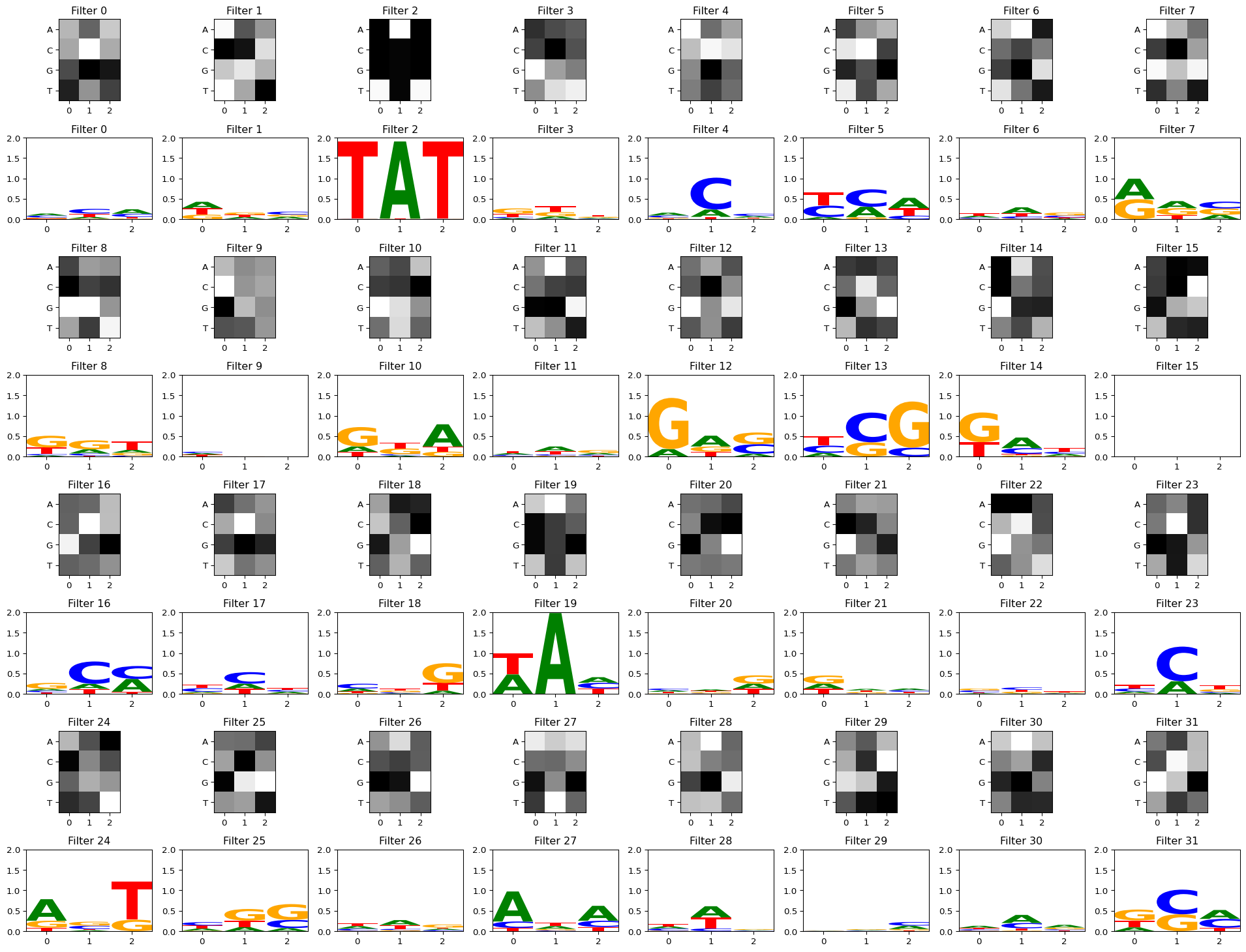

With a stronger activation threshold

Setting act_thresh=1 keeps only the strongest activations, making the logos crisper. Some filters may have no matches above this threshold.

filter_activations = get_filter_activations(some_seqs, conv_layers[0], act_thresh=1)
view_filters_and_logos(model_weights, filter_activations)

Num filters: 32, filter width: 3

/Users/haekyungim/miniconda3/envs/gene46100-dna-cnn/lib/python3.12/site-packages/logomaker/src/Logo.py:1001: UserWarning: Attempting to set identical low and high ylims makes transformation singular; automatically expanding.
  self.ax.set_ylim([ymin, ymax])
/Users/haekyungim/miniconda3/envs/gene46100-dna-cnn/lib/python3.12/site-packages/logomaker/src/Logo.py:1001: UserWarning: Attempting to set identical low and high ylims makes transformation singular; automatically expanding.
  self.ax.set_ylim([ymin, ymax])
/Users/haekyungim/miniconda3/envs/gene46100-dna-cnn/lib/python3.12/site-packages/logomaker/src/Logo.py:1001: UserWarning: Attempting to set identical low and high ylims makes transformation singular; automatically expanding.
  self.ax.set_ylim([ymin, ymax])
/Users/haekyungim/miniconda3/envs/gene46100-dna-cnn/lib/python3.12/site-packages/logomaker/src/Logo.py:1001: UserWarning: Attempting to set identical low and high ylims makes transformation singular; automatically expanding.
  self.ax.set_ylim([ymin, ymax])
/Users/haekyungim/miniconda3/envs/gene46100-dna-cnn/lib/python3.12/site-packages/logomaker/src/Logo.py:1001: UserWarning: Attempting to set identical low and high ylims makes transformation singular; automatically expanding.
  self.ax.set_ylim([ymin, ymax])
/Users/haekyungim/miniconda3/envs/gene46100-dna-cnn/lib/python3.12/site-packages/logomaker/src/Logo.py:1001: UserWarning: Attempting to set identical low and high ylims makes transformation singular; automatically expanding.
  self.ax.set_ylim([ymin, ymax])
/Users/haekyungim/miniconda3/envs/gene46100-dna-cnn/lib/python3.12/site-packages/logomaker/src/Logo.py:1001: UserWarning: Attempting to set identical low and high ylims makes transformation singular; automatically expanding.
  self.ax.set_ylim([ymin, ymax])
/Users/haekyungim/miniconda3/envs/gene46100-dna-cnn/lib/python3.12/site-packages/logomaker/src/Logo.py:1001: UserWarning: Attempting to set identical low and high ylims makes transformation singular; automatically expanding.
  self.ax.set_ylim([ymin, ymax])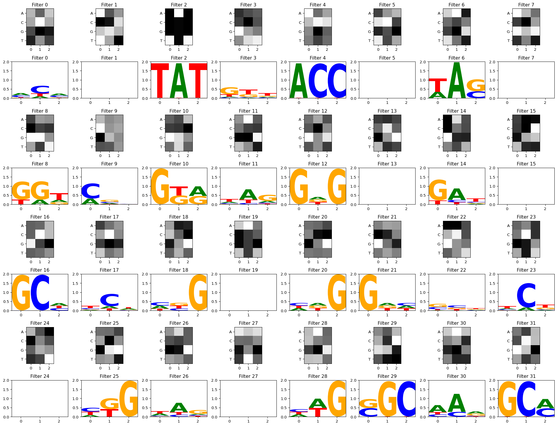

Discuss: You should see some filters that clearly learned TAT and GCG, while others capture subtler nucleotide preferences. In deeper models with multiple conv layers, first-layer filters can combine in complex ways, so they may not always correspond to recognizable motifs (Koo and Eddy, 2019).

Summary

This notebook showed the full pipeline from DNA sequences to trained CNN:

Step	What we did	Why
Scoring rule	Designed a synthetic task with motif bonuses	Verifiable ground truth before tackling real biology
One-hot encoding	A/C/G/T → 4-channel input	Conv1d needs numeric input; 4 channels = 4 nucleotides
DataLoader	Batched training with Dataset + DataLoader	Scales to datasets too large for memory
Linear vs CNN	Compared a position-only model to a motif-capable model	Shows that local context (convolution) is essential for motif detection
Scatter plots	Predicted vs actual scores on held-out test set	Honest evaluation; reveals systematic errors
Filter → logo	Visualized what each filter learned as a sequence logo	Interpretability — do learned filters match known motifs?

Further reading

Foundational papers on CNNs applied to DNA:

• DeepBind: Alipanahi et al 2015
• DeepSEA: Zhou and Troyanskaya 2015
• Basset: Kelley et al 2016

© HakyImLab and Listed Authors - CC BY 4.0 License